10 Best Excel formula to save your time

I am bringing to you some of the most useful formulas and function in the Microsoft Excel. Here is the list of the most helpful Excel formula and function with examples.

What we learn here:

1. What is function and formula in excel?

2. How to create formula OR function in excel?

3. List of the most helpful Excel formula and function with examples.

• SUM() function in excel
• Average function in excel
• If function in excel
• MAX and MIN function in excel
• TRIM function in excel
• Concatenate in excel
• COUNT function in excel
• COUNTIF() Function in excel
• Counta in Excel
• COUNTIFS Function in excel

4. Quiz on function and formula in excel (🏆 Challenge!)

What is function and formula in excel?

We can perform any calculation in excel, using Formulas and Functions. 
So, what is Formulas in excel?, Here, is the answer.
A Formula is simply an equation created by a user in Excel.
And Function in excel ??? 
A Function is a predefined calculation (Function name) in the excel (Spreadsheet).

Function and formula in excel can be used separately or combination of both to solve more complex task in excel.

How to create formula OR function in excel?

In excel you just need to type an equal (=) sign in a cell to create formula. To implement function you need to type equal(=) sign and type predefined calculation (Function name).

Here is the Example of Formula:

=4+3

=C2+C3

Here, is the Examples of a Function:

=SUM(C3:C7)

=MAX(C3:C7)

Hope, You get little bit idea about formula and function.

Hold on, we are jumping on the main topic what you want to learn. I am talking about Excel formula and Excel function. Here we Go to see, How Excel formula can save your time?

List of the most helpful Excel formula and Excel function with examples.

1. SUM() function in excel: 

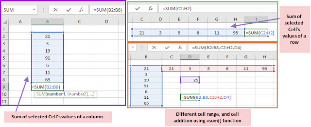
This excel function used to add value of selected cell. The SUM function in excel adds values. You can add individual values, cell ranges or above all together.

Syntax:

=SUM(number1, [number2], …)

Example:

=SUM(B2:B8)  : This will sums the selected Cell's values of a column. Here, Selection range is B2:B8.

=SUM(B2:H2) : This will sums the selected Cell's values of a row. Here, Selection range is B2:H2

=SUM(B2:B8, C9, B2:H2) :  SUM with individual cells, or cells Ranges.

To find average using  SUM() function in excel: 

For example, if you want to find average of 5 different value, then you can find average by using sum() function as given,

=SUM(B2:B6)/5

2. Average function in excel : =AVERAGE()

The average function in excel will return the average of selected cell’s range. You can use the average function to calculate the average. For example if range B1: B10 includes numbers, then the formula =AVERAGE(B1: B10) will return the average of numbers in selected cell’s range.

Syntax of Average function:

=AVERAGE(number1, [number2], ...)

How to use average function in excel ?

Here is the example of average function.

=AVERAGE(B2:B8): Average of the numbers in cells B2 through B8.
=AVERAGE(B2:B8, 10): Average of the numbers in cells B2 through B8 and the number 10.
=AVERAGE(B2:G2) : Average of the numbers in cells A2 through G2.

3. If function in excel (Conditional Formulas in Excel):

what is If function in excel ?

If function in excel, allows to make logical comparisons between any two value. The best part of the IF function in excel is that, you can combine formulas and function both in it.

Syntax of If function in excel:

=IF(logical-test, [value-if-true], [value-if-false])

In given If function syntax : 

• logical-test -  This part of syntax contain a value or condition or logic expression, that can be evaluated as TRUE or FALSE.
• value-if-true - If logical-test is true, then this part of syntax will return.
• value-if-false - If logical-false is false, then this part of syntax will return.

Example of If function in excel:

=if(7>6,”7 is grater value”, “6 is greater value”)

In above if function example, logical-test is 7>6, as you can see this logical-test is true, so the first part “7 is grater value” will be return.

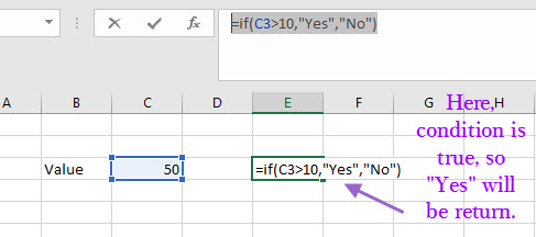
Simple If function in excel with Example:

In simple If function in excel, it checks whether a condition is true or false, and returns one value if true and another value if false.

Simple if function example:

If we have to check value in given cell is greater value then 10 or not. For that, you have to select any cell in excel sheet, where you want comparison and type if function as =if(C3>10,"Yes","No"). 

In above image you can see, if the value is greater than 10, then IF function returns Yes, else it returns No.

And function with if function in excel

If you want to combine more then one condition/logical-test and want result on the basis of if all conditions are true or if any one condition doesn’t meet. Then, AND function in excel with if function will be used. In If function if all conditions are true then, true value part will be return. If any one out of all condition doesn't meet, then False value part will be return.

Let’s take an example, suppose you have to declare result of students as “Pass” or “Fail”. Now, here if student successfully get marks more then, 40 in each subject then only he/she will be declared as “Pass”. If student fail to score more then 40 marks in any single subject then student will be declared as fail.

For that, you can combine if function with And function in excel as below:

=IF(AND(C3>40,C4>40,C5>40),"Pass","Fail")

Here, if function with And  function will combine three conditions to check, Pass or Fail. If all Condition are true, then this formula return "Pass" else return "Fail"

Or Criteria with if function in excel

If you want to combine more than one condition/logical-test and want result on the basis of, If at least one conditions should be true, then Or function in excel with if function can be used.

Let’s take an example, suppose you have to declare student as “Eligible for admission” or “Not Eligible for admission” For next year admission. Now, whether the student scored more than or equal to 70 percentage points in the previous year, or scored more than or equal to 60 marks in the entrance exam, then only qualified for next year admission in a particular branch / stream. 

This means that one should satisfy at least one condition, so in this scenario you can use Or function with if function in excel.

For that, you can combine Or function with If function in excel as below:

=IF(OR(C2>=70, D2>=60)," Eligible for admission "," Not Eligible for admission ")

Here, if function with OR function will combine two conditions to check, eligibility for next year admission. 

If any one out of two Condition are true, then this formula return " Eligible for admission" (Part of syntax when condition is true) else return " Not Eligible for admission " (Part of syntax when condition is false).

Nested If in excel:

If you have to compare more than one value, that means you have multiple conditions to check against one value. Then Nested if (if function within if function) in excel can be used.
For example, if you have to give grade like A,B,C,D according to students performance. In this scenario you have to compare students score with grades like A,B,C,D etc. So, if score >=40 then D grade, if score >=50 then C grade, if score >=65 then B grade, if score >=80 then D grade. To evaluate this given problem in excel you can use nested if like this

=IF(C3>=85,"A",IF(C3>=65,"B",IF(C3>=50,"C",IF(C3>=40,"D","NEED IMPROVEMENT"))))

4. MAX and MIN function in excel

The MAX functions in excel can be used to find the maximum number in a range of values.

The MIN functions in excel can be used to find the minimum number in a range of values.

Example of max() and min() function in excel:

=MAX(C3:C6)   - This will return maximum value from selected range.

=MIN(C3:C6)    - This will return minimum value from selected range.

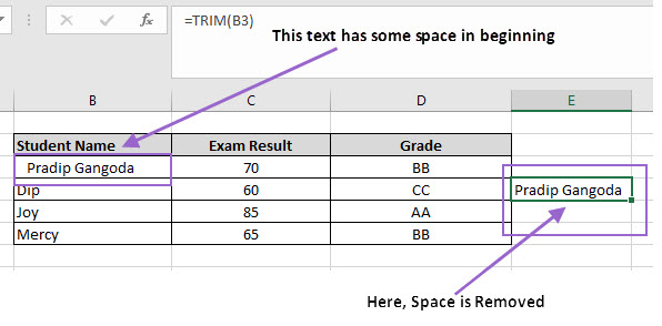
5. TRIM function in excel:

This will remove all spaces form a text string except for single spaces between words.

Example:

=TRIM(B3)

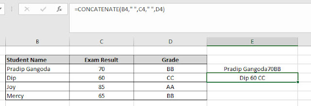
6. Concatenate in excel:

To combine only the contents of cells, this concatenate function in excel is used.

Syntax:

= CONCATENATE(text1, [text2], …)

Example of concatenate excel function

=CONCATENATE(B3,C3,D3)  - This will concatenate content of cells.

=CONCATENATE(B4," ",C4," ",D4)   - This will concatenate contents and add space using “ “ in-between concatenate.

7. COUNT function in excel

The COUNT function in excel counts the number of cells that contain numbers.

Syntax of COUNT function: 

=COUNT(value1, [value2], …)

Example of COUNT  function in excel: 

Let’s take an example, you have a column with mobile no field. And you want to count how many entries are done in that column. For that  you can enter the following formula to count the entries. Suppose the cell’s range of that column is  (B2:B12), So COUNT FUNCTION =COUNT(B2:B12) will give total entries in this range(B2:B12). 

In this example, if all cells range contain numbers, then count function will return total count of cells which contains number. See in given image.

How to use count function in excel?  Here are the steps. 

Step 1: Enter the data(Here mobile number is data) In excel sheet.

Step 2: Select the cell where you want the total count of cells that contain numbers. And enter COUNT FUNCTION like this =COUNT(B2:B12) put cells range in bracket.

Then, Press the Enter key, to complete the formula. And Result will be 6, the count of cells that contain numbers.

This function will count cells that contain only a number. COUNT FUNCTION will not count cells with text value.

8. THE COUNTIF() Function in excel with Example:

To count the number of cells that meet a criterion COUNTIF() function is used. for example, to count the number of times a particular character or place name appears in a list. Only one criteria and only one range are used in COUNTIF() function.

Syntax of countif() function:

=COUNTIF(Range, Criteria)

How to use the COUNTIF() function in Excel ?

Here is the Example of countif function in excel. Let's take an excel sheet, with List of absent and present students. And we want the total count of absent student and total count of present student. In this scenario  COUNTIF() Function come into action.  
This countif function =COUNTIF(D3:D8,"Present")  will give count of present student in D3:D8 cell range.

9. What is Counta in Excel?

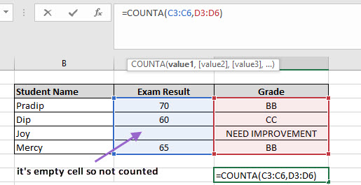
COUNTA function in excel counts all non-empty cells in a given rage. However, it counts all cells regardless of type, that means it counts cells that contain numbers, text, logical values, error values.

Syntax of counta in excel:

=COUNTA (value1, [value2], ...)

Arguments in syntax:

• value1 - An item, cell reference, or range.
• value2 - [optional] An item, cell reference, or range.

Example of counta in excel: 

=COUNTA(C3:C6,D3:D6)

10. COUNTIFS Function in excel

If we have more than one criteria, then countifs function in excel will come into action. Excel COUNTIFS() function returns the cell count that meet one or more criteria. Remember that Each range must have the same number of rows and columns. Empty cell in Range will be treated as a zero value (0).

Syntax of countifs function:

=COUNTIFS(Range1, criteria1, [Range2, criteria2]…)

Syntax arguments:

Range1: The first range in which to evaluate the associated criteria.(Required)

criteria1 : The criteria used to determine which cells to count. criteria1 is applied against range1. (Required)

Range2: The second range in which to evaluate the associated criteria.(Optional)

Criteria2 : The criteria2 used to determine which cells to count in Range2. Criteria2 is applied against range2. (Optional)

How to use countifs in excel ?

Example:
To understand COUNTIFS() we take students marks and grade. And we need number of students with greater or equal to 65 marks and with BB grade.

For that countifs formula is like this:

=COUNTIFS(C3:C6,">=60",D3:D6,"=BB")

This formula will return student with >=60 marks and with "BB" grade

---

Let's Face the Challenge ! - Quiz on Excel Functions

Let's Play Quiz!
Click here

---

For more Microsoft Excel MCQ Practice Click here to get Computer Bits android app

How many sheets are there in ms-excel 2010 workbook by default? - Three

Hope you find this list very helpful to master excel. Happy Learning.