How to use the VLOOKUP excel function ? - Easy Example

Here you will learn VLOOKUP function in excel with easy to follow examples.

What we learn here:

- What is vlookup function in excel ?
- Examples of vlookup function in excel.
- A lookup value that does not exist with TRUE and FALSE fourth argument in vlookup function.
- What to Do if You're Getting an #N/A Error with VLOOKUP excel function.

What is vlookup function in excel ?

VLOOKUP in excel helps you to check your tablet for specific information in excel spreadsheet. For example, if you have a Student Result list, and you want to look at the total marks of any specific student. Here, You can use the VLOOKUP. VLOOKUP Function in excel is very beneficial on larger and more complicated tables.

Before we learn how to use VLOOKUP FUNCTION in excel. Let’s understand syntax of vlookup.

Syntax of vlookup in excel:

=VLOOKUP(LookupValue, TableArray, ColumnIndexNumber, FALSE/TRUE)

Arguments in vlookup syntax:

LookupValue: 

The value, that you want to look up. (value to lookup, must be in left most column in selected table range.)

TableArray: 

The table where you want to find value (The Table taken in second argument in syntax).

ColumnIndexNumber: The column number in Table. (The column number in selected table, third argument).

FALSE or 0/TRUE or 1:
FALSE or 0 tells the VLOOKUP function to return an exact match.
The lookup range can be in of any order. Vlookup will return a value from the first row where the lookup value is equal to any value from selected range value. If no rows meet this criterion then #N/A error is returned.
TRUE or 1 tells the VLOOKUP function to return an approximate match. The lookup range is mostly in ascending order from top to bottom. Vlookup will return the last row where the range value is lessthen or equalto (<= ) the lookup value. If no rows meet this criteria then #N/A error is returned.

As shown in above Syntax you need four arguments to create VLOOKUP function in excel.

1. LookupValue

2. TableArray

3. ColumnIndexNumber

4. Flase/True. 

Example of vlookup function in excel. ( How to use vlookup function in excel ? )

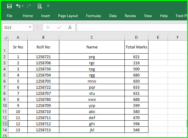
Here is the easy to learn, step by step vlookup examples. Let’s Take some data in excel spread sheet as shown below:

From above data suppose you want total marks of rollno 1258721 for that you have to build vlookup function as:

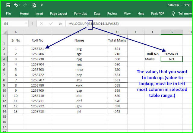
=VLOOKUP(G3,B2:D14,3,FALSE)

Let's understand arguments in above syntax.

First argument in vlookup formula in excel:

In vlookup formula =VLOOKUP(G3,B2:D14,3,FALSE), the first argument is the value for lookup. Here in excel sheet we put value to lookup in G3 cell as shown in above image. And lookup value is 1258721. Value to lookup, must be in left most column in selected table range.

Here if vlookup formula =VLOOKUP(1258721,B2:D14,2,FALSE) will return prg as column index is 2.

Here if vlookup formula =VLOOKUP(1258720,B2:D14,2,FALSE) return #N/A error as lookup value is not found(no exact match found) in selected range(left most column).

Second argument in vlookup formula in excel:

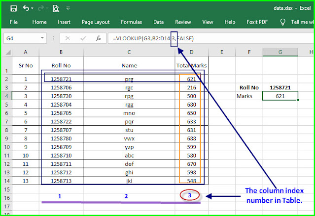
In vlookup formula =VLOOKUP(G3,B2:D14,3,FALSE), the second argument is the table where we have to lookup value. Here in excel sheet selected table range is B2:D14. Keep in mind that the lookup value must be in first column of selected table as shown in image.

Third argument in vlookup formula in excel:

In vlookup formula =VLOOKUP(G3,B2:D14,3,FALSE), the third argument is the column index number. Here in excel sheet we want total marks(third column of selected table) for lookup value(1258721) so third argument is 3.

Fourth argument in vlookup formula in excel:

In vlookup formula =VLOOKUP(G3,B2:D14,3,FALSE), the  Fourth argument may be TRUE/FALSE. FALSE tells the VLOOKUP function to return an exact match. TRUE tells the VLOOKUP function to return an approximate match(Close value). Here in excel sheet we want exact match, so we have fourth argument is FALSE as shown in image.

Let's take a lookup value that does not exist in our excel sheet data with FALSE as fourth argument.

As lookup value we take here is 1258720 which is not available in left most column of selected table. So vlookup function will return #N/A error.

Let's take a lookup value that does not exist in our excel sheet data with TRUE as forth argument.

As lookup value we have taken here is 1258720, which is not available in left most column of selected table. In first column in selected table range lookup value 1258720 is not found. so vlookup function with true as last argument will return the last row value, which is less then or equal to the lookup vlaue. And here, 1258713 is the last row with lessthen the lookup value 1258720.

What to Do if You're Getting an #N/A Error with VLOOKUP excel function.

The #N/A Error in vlookup function means that a function can not find what it needs to find.
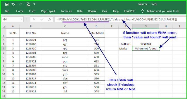
OK, so your function does not found what you want and return that traditional excel error #N/A. Don’t worry you can customize this vlookup function, so you will get your customize message when value is not found..

To do so you can your If function in excel.

=IF(ISNA(VLOOKUP(1258720,B2:D14,3,FALSE )),"Value not found",VLOOKUP(1258720,B2:D14,3,FALSE ))

OR

=IFNA(VLOOKUP(1258720,B2:D14,3,FALSE ),"Value not found")

OR

=IFERROR(VLOOKUP(1258720,B2:D14,3,FALSE ),"Value not found")

As lookup value we take here is 1258720 which is not available in left most column of selected table. So vlookup function will return #N/A error. And using above three if, ifna and iferror function you will return customize error in excel.

I am sure, you've find this vlookup in excel post helpful in your excel learning journey. If you have any question or query, then leave in comment section. Keep Learning and Keep Sharing!