Today, with a very clear and easy example, we will learn how to build a drop-down list in Excel. We are going to do this using the Data Validation feature offered by Excel.
- We'll now build the drop-down list in excel - First way
- Another simple way to create a Dropdown list, by typing the list in the source box.
- Allow Other Entries in the dropdown list in excel.
- How to Add/Remove Items in the dropdown list in excel?
- Dynamic Drop-down List in excel using OFFSET() function.
- How to Remove a Drop-down List in excel.
- Create Dependent Drop-Down Lists in Excel Using OFFSET() and MATCH() excel Function. 👈
We'll now build the drop-down list in excel.
Follow the easy steps:
Step 1:
Create Item List with a header, Create a list of Items with a header in another sheet. Here we create a semester list in sheet 2. See the image below to get an idea about the list.
The list contains Semester 1, Semester 2, Semester 3, Semester 4, Semester 5, Semester 6, and header name Semester. See in Image above.
Step 2:
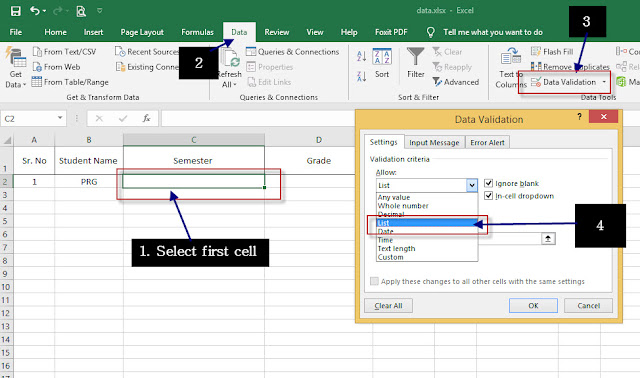
Create the Drop Down list in excel, Go to sheet1 where, you want to create a dropdown list to fill in data. Here in sheet1 go to Data Tab > Select column range where you want to create a dropdown list > Click on Data Validation
Step 3:
In the appeared Data Validation Window, From the Allow drop-down list, choose List.
Step 4:
Then, in the appeared Data Validation window, In the source box, you have to give a range of item lists, which you want to see in the dropdown.
In our example we have created an item list in sheet2, so select/Click in source textbox and go to sheet2 and select cell range with item list. See in Image below.
Another simple way to create a Dropdown list, by typing the list in the source box.
Step 1:
Go to the excel sheet where you want to create a dropdown list to fill in data. Select column range where you want to create a dropdown list.
Step 2:
Here in sheet1 go to Data Tab.
Step 3:
Click on Data Validation
Step 4:
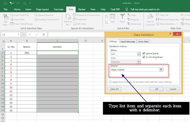
In the appeared Data Validation Window, From the Allow drop-down list, choose List
Then, in the appeared Data Validation window, in the source box, you have to type the item list, which you want to see in the dropdown. Type list item in the source box and separate each item with a delimiter.
Step 6:
Click Ok.
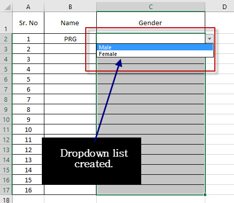
Here is the created
dropdown list in excel.
Allow Other Entries in the dropdown list in excel.
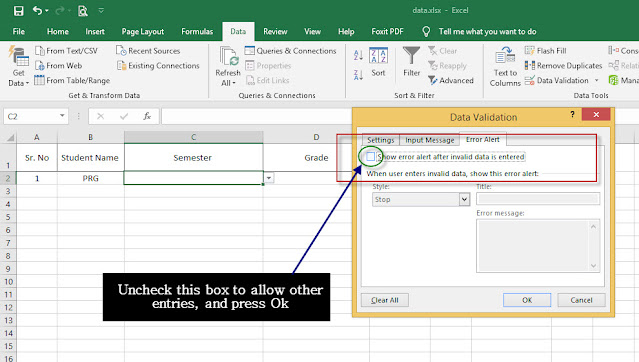
You can also create a drop-down list in Excel that allows other entries. If you type a value that is not on the list, Excel shows an error alert as shown in the image below.To allow other entries, execute the following steps.
Step 1: Go to the excel sheet where you want to create a dropdown list to fill in data. Here in sheet1 go to Data Tab > Select column range where you want to create a dropdown list.
Step 2:
Click on Data Validation.
Step 3:
In the appeared Data Validation Window, On the Error Alert tab, uncheck 'Show error alert after invalid data is entered'.
Step 4:
Then click Ok.
Now you can enter the item, which is not available in the dropdown list in excel.
How to Add/Remove Items in the dropdown list in excel?
- Add item in between other items in the item list so you don’t need to change the cell range in Data Validation Window. Don’t add items at the last location in the list.
- To remove an item from a drop-down list, just delete item value from the item list.
Dynamic Drop-down List in excel using OFFSET() function
Go to the excel sheet, where you want to create a dropdown list in excel. Select the first cell where you want to create a dropdown list. Here, in this example, I have selected cell C3.
- In Data Validation Window, Click in the Source box and enter the formula: =OFFSET(ItemList!$B$2,0,0,COUNTA(ItemList!$B:$B),1)
Explanation of offset function in excel:
- The OFFSET function has 5 arguments.
ItemList!$B$2 = Is the first item in the item list
0 = rows to offset
0 = columns to offset
COUNTA(ItemList!$B:$B) = Height.
1 = width.
COUNTA function in excel counts all non-empty cells in a given rage. However, it counts all cells regardless of type, which means it counts cells that contain numbers, text, logical values, error values. When you add an item to the list on the ItemList sheet, COUNTA(ItemList!$B:$B) increases. As a result, the range returned by the OFFSET function expands and the drop-down list will be updated.
Press Ok and Dynamic Drop-Down list is Ready. Now add a new value in the item list, and see that the dropdown list is now updated with the new value.
How to Remove a Drop-down List in excel:
To remove a drop-down list in Excel, execute the following steps.
Step 1:
Select Cell or Cell range with Drop-down List.
Step 2:
On the Data tab, in the Data Tools group, click Data Validation.
Step 3:
The 'Data Validation' dialog box appears.
Step 4:
Click Clear All.
Create Dependent Drop-Down Lists in Excel Using OFFSET() and MATCH() excel Function.
Before we create multiple dependent drop-down lists in excel, let's understand the offset and match function in excel.
=OFFSET() function in excel
Usage:
It aims to return a range specifying the number of rows and columns from a given cell or range.
Syntax:
=OFFSET (reference, rows, cols, [height], [width])
Reference: a starting point/cell or range
Rows: a row offset
Cols: a column offset
Height: height in rows
Width: width in columns.
Match() excel function:
Usage:
It is used to locate the position of a lookup value in a given row range or column range or table.
Syntax:
=MATCH (lookup-value, lookup-array, [match-type])
Lookup-value: The value to match in lookup_array.
Lookup-array: A range of cells or an array reference.
Match-type: 1 or 0 or -1
1 = exact or next smallest (default),
0 = exact match
-1 = exact or next largest
Now we are going to create a dependent drop-down list:
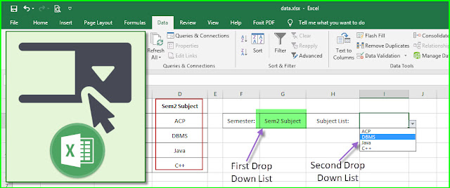
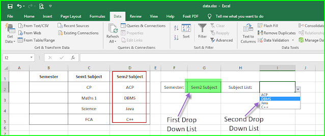
In our example, we are creating two drop-down lists. The First, drop-down list is of semester number and the second drop-down list is of the subject name of the respective semester.
For example, when you select semester 1 then in the second drop-down list you will have a subject list of semester 1. Same way when you select semester 2 then in the second drop-down list you will have the subject list of semester 2.
As shown in the image below creates the first drop-down list in excel:
- To create a dropdown list which depends on the selection of the first dropdown list, follow the steps:
Step 1:
Select the cell where you want to create a second drop-down list.
Step 2:
Go to the Data tab and, in the Data Tools group, click Data Validation.
Step 3:
In the appeared Data Validation Window, From the Allow drop-down list, choose List.
Then, in appeared Data Validation window, In the source box, you have to type
=OFFSET($B$1,1,MATCH($G$2,$C$1:$D$1),4,1) formula.
In this offset formula.
$B$1 is the starting point,
1 is the row offset,
MATCH($G$2,$C$1:$D$1) will return position and this is column offset.
4 is height
1 is the width.
Than you for learning with me. Hope you find this post of how to create a drop-down list in excel very useful. Keep learning keep sharing.








0 Comments